Applications
In this section, applications for different data type are presented; each of them prepare data to suit the conventions used in HyDE package and in FloodPROOFS modelling system too. Once data are collected from different sources, they are available in a raw format and it is necessary to adapt them, for example changing format, resolutions and domain, to the outcome conventions. All applications are stored in the apps folder in the root of the package; an example of apps tree is reported:
hyde-master
├── **apps**
│   ├── ground_network
│   │   ├── rs
│   │   └── ws
│   ├── nwp
│   │   ├── gfs
│   │   ├── lami
│   │   └── wrf
│   ├── rfarm
│   │   ├── lami
│   │   └── wrf
│   ├── satellite
│   ├── utils
│   └── ...
├── bin
├── docs
├── src
│   ├── common
│   └── hyde
├── test
├── AUTHORS.rst
├── CHANGELOG.rst
├── LICENSE.rst
└── README.rst
Ground Network Applications
The procedure of weather stations data, available in HyDE package is divided in two parts:
extraction of weather stations datasets, both for all requested variables and every time step, from an local or worlwide database (using queries or functions developed specifically for that database) and storage of all variables data in a CSV file for each variable and for every timestep;
conversion of stations data, available in the CSV files created previously, in a spatial information over the selected domain (using, for instance, interpolation, regridding or warping methods) and saving all variables in a netcdf4 file for every timestep.
As previously said, the first step of procedure is about the downloading/getting data from a database or data repository. The extraction of weather stations data is performed by an python3 application available in HyDE package in “/hyde-master/bin/downloader/ws/” named “hyde_downloader_{database_name}_ws.py”; for configuring this procedure, a JSON file usually named “hyde_downloader_{database}_ws.json” has to be filled in all of its part. The name of used database has to be specified by the users according with their settings. At the end, a output CSV file will be created with all data for each variable and for every timestep.
General use of the weather stations downloader is reported below:
>> python3 hyde_downloader_ws.py -settings_file hyde_configuration_ws.json"
In the next example, the settings of downloading procedure for rain data is reported. Users can activate downloading of selected variable using attribute “download” equal to “true”. The units of the variable can be specified in order to save this information in the CSV file.
"rain": {
    "download": true,
    "name": "Rain",
    "sensor": "Raingauge",
    "units": "mm"
},
According with the period of simulation or analysis, the time fields have to be updated. Frequency and expected data period have to be set by the users.
"time_info": {
    "time_get": "201809010500",
    "time_period": 6,
    "time_frequency": "H"
},
Once source data are configured, the weather stations data will be save in a CSV file.
The second step of procedure concerns the spatialization of weather stations data. Spatial datasets of weather stations data are realized using an python3 application available in HyDE package in “/hyde-master/apps/ground_network/ws/” named “HYDE_DynamicData_GroudNetwork_WS.py”; for configuring this procedure, a JSON file usually named “hyde_configuration_groundnetwork_ws.json” has to be filled in all of its part. Starting from CSV file previously created, the script will able to save an netCDF4 output file will be created with all variables data for every timestep.
General use of the weather stations application is reported below:
>> python3 HYDE_DynamicData_GroundNetwork_WS.py -settings_file hyde_configuration_groundnetwork_ws.json -time "%Y-%m-%d %H:%M"
For example, if the application is set to 2016-03-13 22:00:
>> python3 HYDE_DynamicData_GroundNetwork_WS.py -settings_file hyde_configuration_groundnetwork_ws.json -time "2016-03-13 22:00"
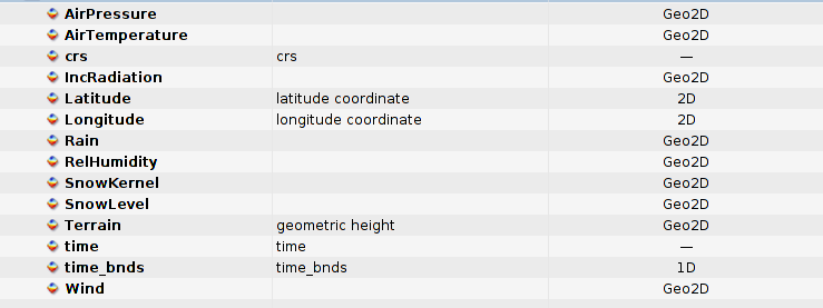
Example of variable list for an weather stations output file.
For example to set the time information, users have to change a time fields according with their simulation settings:
"time": {
    "time_forecast_step": 0,
    "time_forecast_delta": 0,
    "time_observed_step": 10,
    "time_observed_delta": 3600,
    "time_reference_type": {
        "units": null,
        "rounding": null,
        "steps": null
    }
}
All the input variables needed for performing simulation have to be set in dynamic source and outcome fields available in the JSON configuration file. In the next example, rain configurarion options are reported. Users can change, for instance, the interpolation method (for example “nearest”) and interpolation radius influence along x and y. If some variables are not available to avoid warnings and faults, users can be set “var_mode” to “false” in order to save time and skip uncessary elaborations.
"outcome": {
    "rain_data":{
        "id": {
            "var_type": ["var2d", "interpolated"],
            "var_mode": true,
            "var_name": ["Rain"],
            "var_file": "ws_product",
            "var_colormap": "rain_colormap",
            "var_method_save": "write2DVar"
        },
        "attributes": {
            "long_name": "Rain",
            "standard_name": "rain",
            "_FillValue": -9999.0,
            "ScaleFactor": 1,
            "units": "mm",
            "Valid_range": [0, null],
            "description": ""
        }
    },
}
Once source data are configured, outcome data need to be configureted too. Users, for example, can be set units, scale factor and valid range to properly filter weather stations data and define a spatial information that will be saved in a netCDF4 output file.
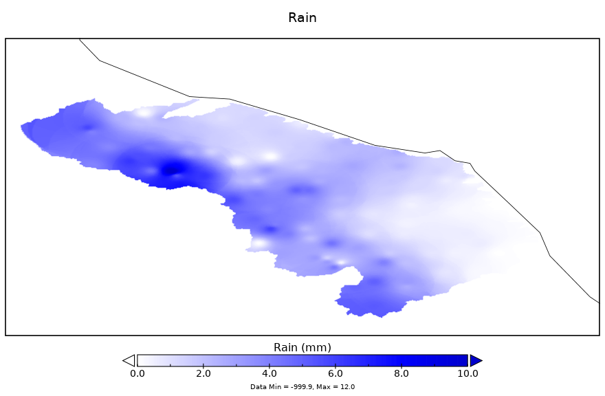
Example of rain map for Marche Italian region.
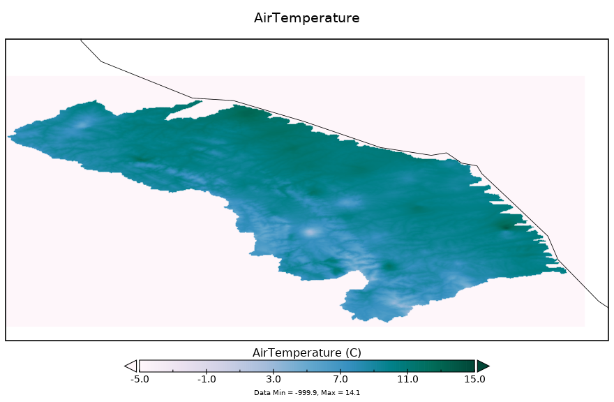
Example of air temperature map for Marche Italian region.
Satellite Applications
H-SAF
The “EUMETSAT Satellite Application Facility on Support to Operational Hydrology and Water Management (H-SAF)” started on 2005 as part of the EUMETSAT SAF Networks. The H-SAF generates and archives high-quality data sets and products for operational hydrological applications starting from the acquisition and processing of data from Earth observation satellites in geostationary and polar orbits operated both by EUMETSAT and other satellite organization. The retrieval of products uses data from microwave and infrared instruments and aims at reaching the best possible accuracy compatible with satellite systems as available today or in the near future. H-SAF applications fit with the objectives of other European and international programmes with special relevance to those initiatives which want to mitigate hazards and natural disasters such as flash floods, forest fires, landslides and drought conditions, and improve water management. All the information about the project and the product are available on HSAF WebSite.
- In H-SAF project the products are divided in three categories:
precipitation (liquid, solid, rate, accumulated;
soil moisture (at large-scale, at local-scale, at surface, in the roots region);
snow parameters (detection, cover, melting conditions, water equivalent).
- In HyDE python package, the following applications are available to perform analysis over these products:
precipitation –> H03b, H05b;
soil moisture –> H14, H16, H101;
snow parameters –> H10, H12, H13.
The procedures of H-SAF consist in some applications written in python3 available in HyDE package in “/hyde-master/apps/satellite/HSAF/”.
The product H03B is based on the IR images from the SEVIRI instrument on-board Meteosat Second Generation (MSG) satellites. The spatial coverage of the product included the H-SAF area (Europe and Mediterranean basin) and the Africa and Southern Atlantic Ocean. Thus the new geographic region covers the MSG area correspondent to 60°S – 67.5°N, 80°W – 80°E.
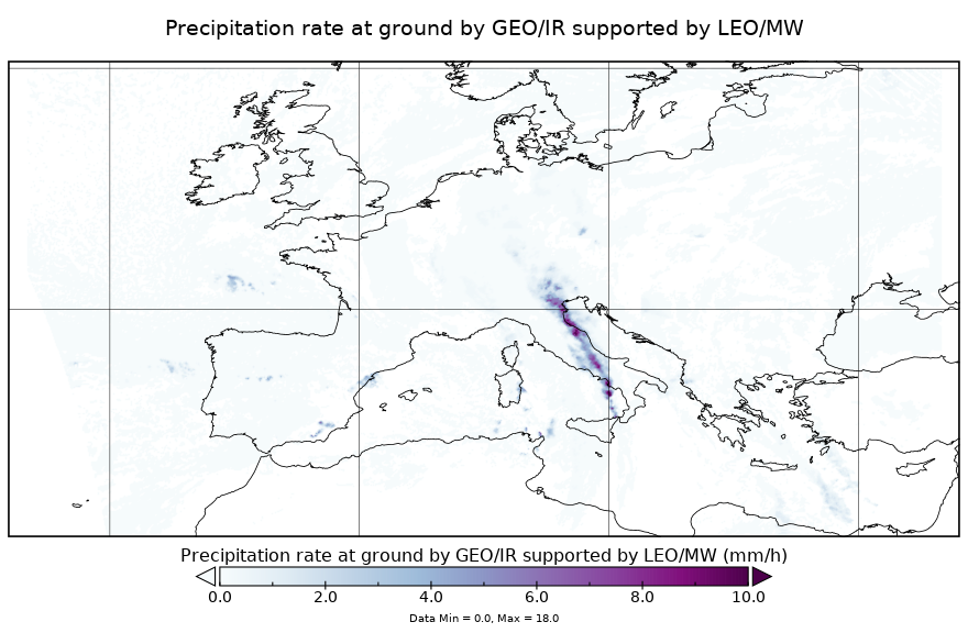
Example of h03b istantaneous rain map for Europe domain.
The product is generated at the 15-min imaging rate of SEVIRI, and the spatial resolution is consistent with the SEVIRI pixel. The precipitation estimates are obtained by combining IR GEO equivalent blackbody temperatures at 10.8 μm with rain rates from PMW measurements. The units of H03b istantaneous rain product are expressed in [mm/h].
General use of the H03B application is reported below:
>> python3 HYDE_DynamicData_HSAF_H03B.py -settings_file configuration.json -time "%Y-%m-%d %H:%M"
The h05b product is derived from precipitation maps generated by merging MW images from operational sun-synchronous satellites and IR images from geostationary satellites. Integration is performed over 3, 6, 12 and 24 hours.
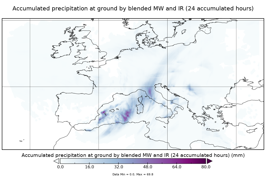
Example of h05b accumulated rain map for Europe domain.
In order to reduce biases, the satellite-derived field is forced to match raingauge observations and, in future, the accumulated precipitation field outputted from a NWP model. The units of H05b accumulated rain product are expressed in [mm].
General use of the H05B application is reported below:
>> python3 HYDE_DynamicData_HSAF_H05B.py -settings_file configuration.json -time "%Y-%m-%d %H:%M"
The H10 product is an output of image classification processing. The snow signature is recognised as differential brightness in more short-wave channels, intended to discriminate snow from no-snowed land and snow from clouds.
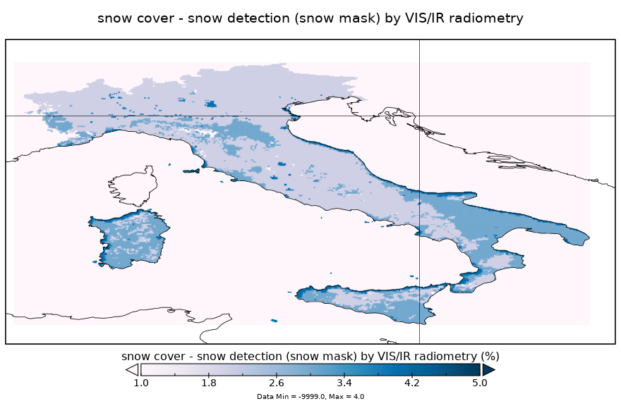
Example of h10 snow cover map for Italy domain, where 1:snow, 2:cloud, 3:bare ground, 4:water, 5:dark/no_data.
Both radiometric signatures are used (specifically, the 1.6 micron channel as compared with others), and time-persistency (for cloud filtering by the “minimum brightness” technique applied over a sequence of images).
General use of the H10 application is reported below:
>> python3 HYDE_DynamicData_HSAF_H10.py -settings_file configuration.json -time "%Y-%m-%d %H:%M"
The H12 product differs from H10 in so far as, in the snow map, the resolution elements report the fractional snow coverage instead of being binary (snow/snow-free). The possibility of appreciating fractional coverage stems from the lack of observed brightness in respect of what would be if the pixel were fully filled by snow..
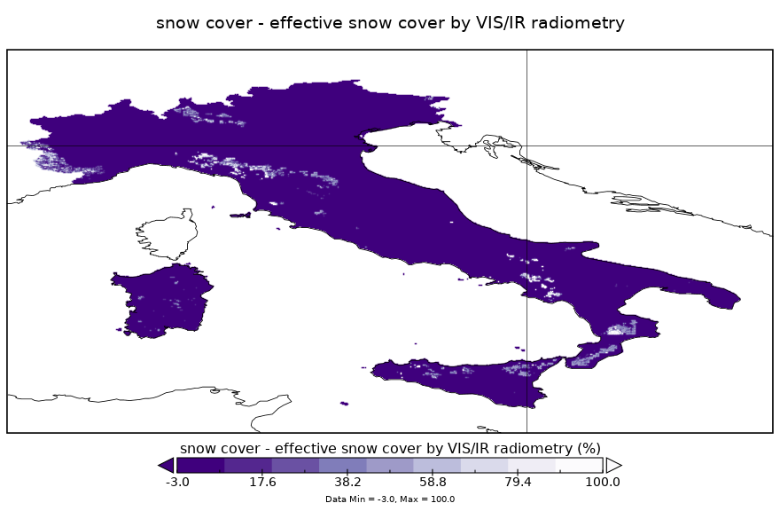
Example of h12 snow cover map for Italy domain, where 0:bare ground, 1-100:fractional cover -1:no_classified/no_data, -2:cloud, -3:water.
The forest canopy obscuring the full visibility to the ground is accounted for by applying certain a priori transmissivity information, which must be generated using satellite-borne reflectance data acquired under full dry snow cover conditions
General use of the H12 application is reported below:
>> python3 HYDE_DynamicData_HSAF_H12.py -settings_file configuration.json -time "%Y-%m-%d %H:%M"
The H13 product is generated by using microwaves that are sensitive to snow thickness and density, i.e. to the snow water equivalent. Depending on the snow being dry or wet, the penetration changes (dry snow is more transparent). High frequencies are required for dry snow, which is an advantage from the resolution viewpoint.
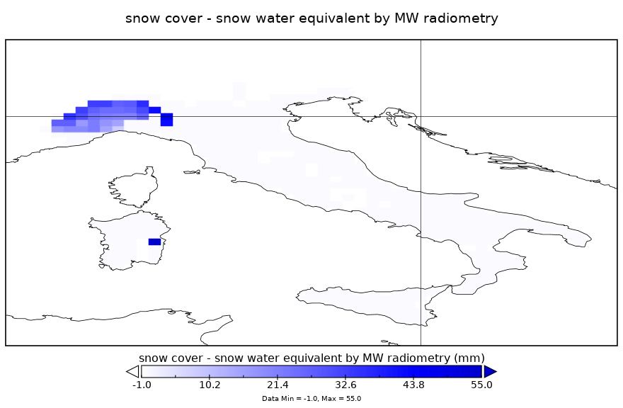
Example of h13 snow water equivalent map for Italy domain, where 0:bare ground, 1-500:snow water equivalent, -1:no_classified/no_data
However, with increasing snow depth, lower frequencies are necessary for better penetration, thus a multifrequency approach is required. It is an all-weather, night-and-day measurement, whose processing requires considerable support from ancillary information. Method and performance may be different for flat/forested areas and mountainous regions.
General use of the H13 application is reported below:
>> python3 HYDE_DynamicData_HSAF_H13.py -settings_file configuration.json -time "%Y-%m-%d %H:%M"
The Level 2 surface soil moisture products H16 and H101 are derived from the radar backscattering coefficients measured by the Advanced Scatterometer (ASCAT) on-board the series of Metop satellites using a change detection method, developed at the Research Group Remote Sensing, Department for Geodesy and Geoinformation (GEO), Vienna University of Technology (TU Wien).
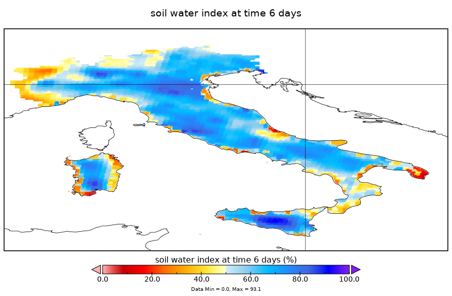
Example of ASCAT H16/H101 soil water index (SWI) map, based on surface soil moisture (SSM) time-series.
In the TU Wien soil moisture retrieval algorithm, long-term Scatterometer data are used to model the incidence angle dependency of the radar backscattering signal. Knowing the incidence angle dependency, the backscattering coefficients are normalized to a reference incidence angle. Finally, the relative soil moisture data ranging between 0% and 100% are derived by scaling the normalized backscattering coefficients between the lowest/highest values corresponding to the driest/wettest soil conditions. Once SSM values are obtained, next step is how to extend the influnce of SSM at the different soil deepths. Starting from the SSM values, the Soil Water Index (SWI) is a method to estimate root zone soil moisture using an exponential Filter.
The ASCAT OBS applications, based on H16 and H101 products, are developt in order to compute the time-series of SSM and SWI both for the data record (DR) and the near-real-time (NRT) datasets.
General use of ASCAT OBS application for computing data record dataset is reported below:
>> python3 HYDE_DynamicData_HSAF_ASCAT_OBS_DR.py -settingfile configuration_product.json
For computing the near-real-time datasets, the genearal command-line is as follows:
>> python3 HYDE_DynamicData_HSAF_ASCAT_OBS_NRT.py -settingfile configuration_product.json -time "%Y-%m-%d %H:%M"
The product H14 is generated by the soil moisture assimilation system, using the surface observation from ASCAT that is propagated towards the roots region down to 2.89 m below surface, providing estimates for 4 layers (thicknesses 0.07, 0.21, 0.72 and 1.89 m). The ECMWF model generates soil moisture profile information according to the Hydrology Tiled ECMWF Scheme for Surface Exchanges over Land (HTESSEL). The product is available at a 24-hour time step, with a global daily coverage at 00:00 UTC.
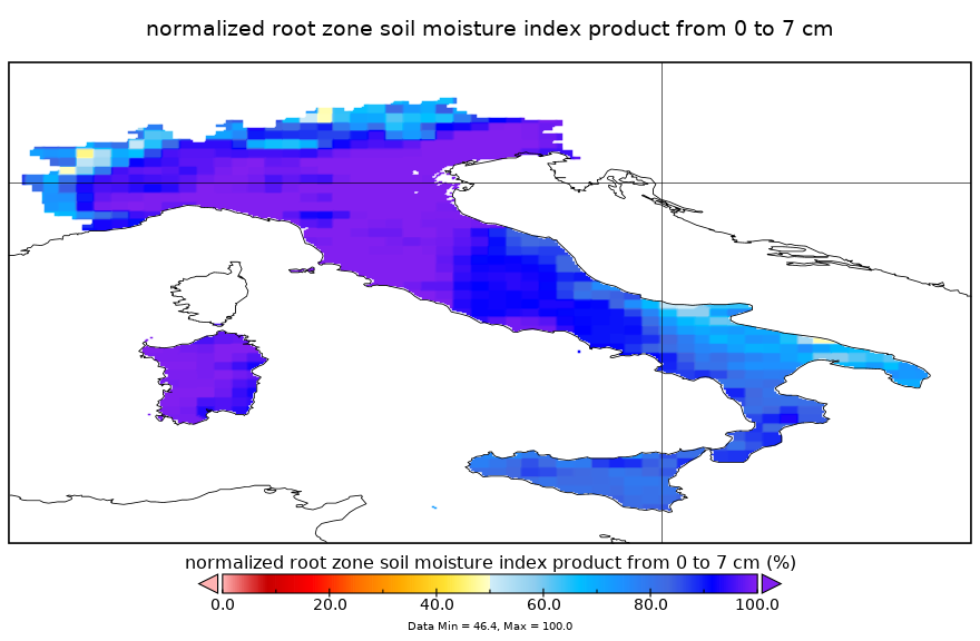
Example of ASCAT H14 root zone soil moisture 0 - 7 cm.
The product H14 is produced in a continuous way in order to ensure the time series consistency of the product (and also to provide values when there is no satellite data, from the model propagation). The SM-DAS-2 product is the first global product of consistent surface and root zone soil moisture available NRT for the NWP, climate and hydrological communities.
The ASCAT MOD applications, based on H14 product, are developt in order to compute the time-series of SSM and SWI both for the data record (DR) and the near-real-time (NRT) datasets.
General use of ASCAT MOD application for computing data record dataset is reported below:
>> python3 HYDE_DynamicData_HSAF_ASCAT_MOD_DR.py -settingfile configuration_product.json
For computing the near-real-time datasets, the genearal command-line is as follows:
>> python3 HYDE_DynamicData_HSAF_ASCAT_MOD_NRT.py -settingfile configuration_product.json -time "%Y-%m-%d %H:%M"
The configuration files for all H-SAF products have to be filled in order to correctly set the algorithms.
MODIS
The MODIS Snow Cover products are generated using the MODIS calibrated radiance data products (MOD02HKM and MYD02HKM), the geolocation products (MOD03 and MYD03), and the cloud mask products (MOD35_L2 and MYD35_L2) as inputs. The MODIS snow algorithm output (MOD10_L2 and MYD10_L2) contains scientific data sets (SDS) of snow cover, quality assurance (QA) SDSs, latitude and longitude SDSs, local attributes and global attributes. The snow cover algorithm identifies snow-covered land; it also identifies snow-covered ice on inland water. Further information are available on MODIS Snow Cover WebSite.
General use of MODIS Snow Cover application is reported below:
>> python3 HYDE_DynamicData_MODIS_Snow.py -settingfile configuration_product.json
Numerical Weather Prediction Applications
Deterministic mode
The procedure of numerical weather prediction data consists in an application written in python3 available in HyDE package in “/hyde-master/apps/{nwp_name}” named “HYDE_DynamicData_NWP_{nwp_name}.py”; for configuring this procedure, a JSON file usually named “hyde_configuration_nwp_{nwp_name}.json” has to be filled in all of its part. For example, in case of wrf is used the name of the HyDE application will be updated using “wrf” to complete names of folders, procedures and configuration files.
General use of the nwp application is reported below:
>> python3 HYDE_DynamicData_NWP_{nwp_name}.py -settings_file hyde_configuration_nwp_{nwp_name}.json -time "%Y-%m-%d %H:%M"
For example, if the application is about wrf at 2019-05-22 13:00:
>> python3 HYDE_DynamicData_NWP_WRF.py -settings_file hyde_configuration_nwp_wrf.json -time "2019-05-22 13:00"
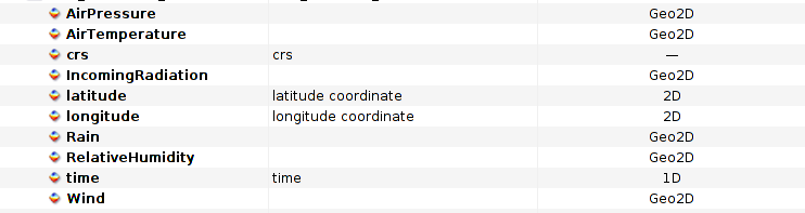
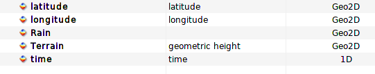
Example of variable list for an nwp output file.
In the configuration file, users can change settings of variables and timing information. Time fields have to be changed according with nwp timestep resolution and forecast length.
"time": {
  "time_forecast_step": 48,
  "time_forecast_delta": 3600,
  "time_observed_step": 0,
  "time_observed_delta": 0
},
About variables and their attributes, users can update name, type and computational methods of each variable. Scale factor, units, missing value and fill value are requested to get and filter values.
"air_temperature_data": {
  "id": {
    "var_type": ["var3d", "istantaneous"],
    "var_name": ["T2"],
    "var_file": "wrf_data",
    "var_method_get": "get2DVar",
    "var_method_compute": "computeAirTemperature"
    },
  "attributes": {
    "ScaleFactor": 1,
    "Missing_value": -9999.0,
    "_FillValue": -9999.0
    }
}
Output format and features of the variable have to be set too. The users can specify, for instance, units, format and ancillary variables. The function to write data in netCDF4 format can be changed according with data expected by the other applications in forecasting chain.
"air_temperature_data":{
  "id": {
    "var_type": ["var3d", "istantaneous"],
    "var_name": "AirTemperature",
    "var_file": "wrf_product",
    "var_colormap": "air_temperature_colormap",
    "var_method_save": "write3DVar"
    },
  "attributes": {
    "long_name": "",
    "standard_name": "",
    "ancillary_variables": ["T2"],
    "units": "C",
    "Format": "f4",
    "description": "Temperature at 2m"
    }
}
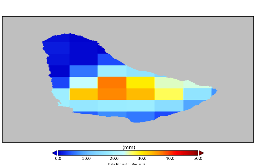
Example of rain map for Barbados island.
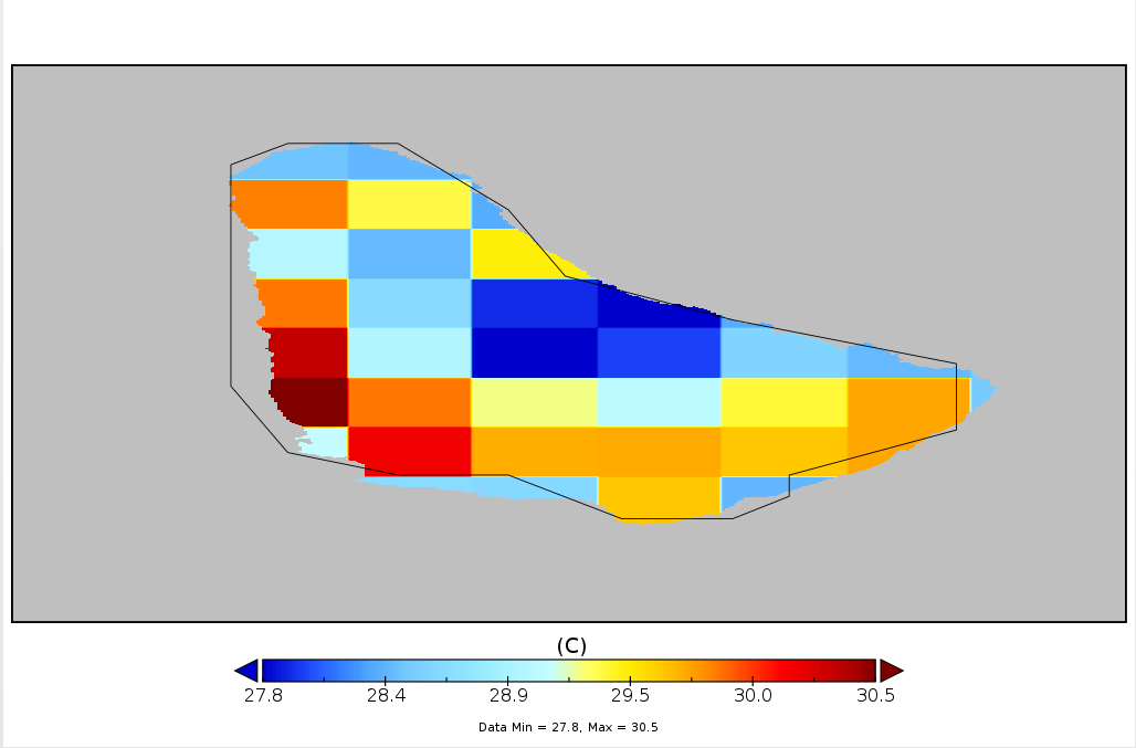
Example of air temperature map for Barbados island.
Probabilistic mode - Rainfarm model
The procedure of Rainfarm model consists in an application written in python3 available in HyDE package in “/hyde-master/apps/rfarm” named “HYDE_Model_RFarm_{nwp_name}.py”; for configuring this procedure, a JSON file usually named “hyde_configuration_rfarm_{nwp_name}.json” has to be filled in all of its part. For example, in case of WRF numerical model is used the name of the HyDE application will be updated using “wrf” to complete names of folders, procedures and configuration files.
General use of the nwp application is reported below:
>> python3 HYDE_Model_RFarm_{nwp_name}.py -settings_file hyde_configuration_rfarm_{nwp_name}.json -time "%Y-%m-%d %H:%M"
For example, if the application is about wrf at 2019-05-22 13:00:
>> python3 HYDE_Model_RFarm_WRF.py -settings_file hyde_configuration_rfarm_wrf.json -time "2019-05-22 13:00"
Example of variable list for an nwp output file.
Obviously, according with NWP version and features, users have to set the reliable spatial scale of LAM Lo (cs_sf in the configuration file) and the reliable temporal scale of LAM T0 (ct_sf in the configuration file). The number of ensembles have to be set, too.
"parameters": {
    "ensemble": {"start": 1, "end": 30},
    "ratio_s": 6,
    "ratio_t": 1,
    "slope_s": null,
    "slope_t": null,
    "cs_sf": 2,
    "ct_sf": 2,
    "multi_core": false,
    "domain_extension": 0,
    "tmp": true
}
In the configuration file, users can change settings of variables and timing information. Time fields have to be changed according with nwp timestep resolution and forecast length.
"time": {
    "time_forecast_period": 48,
    "time_forecast_frequency": "H",
    "time_observed_period": 0,
    "time_observed_frequency": "H",
    "time_rounding": "H"
}
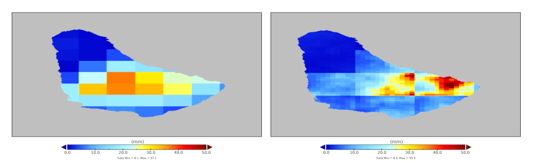
Example of comparison between nwp map and disaggregated map for Barbados island.
Further details on the Rainfarm model are reported in AnnexB.